Motion Graphs and Mathematical Models

Driving question

How can graph shape, slope, area, and residuals turn measurements into a defensible motion model?

Before learning: match the story

A cart moves right, slows uniformly, stops, and then moves left faster and faster. Sketch its position-time, velocity-time, and acceleration-time graphs before reading further. Mark the stopping instant on every graph.

Hook: a graph can predict a measurement you never used

A model becomes useful when it predicts withheld data—not merely when its curve looks smooth. Motion graphs encode rates of change and accumulation, while residuals reveal patterns the fitted equation misses.

Three graphs, one motion

For one-dimensional motion,

Graphically:

• slope of $x$ versus $t$ is velocity;
• slope of $v$ versus $t$ is acceleration;
• signed area under $v$ versus $t$ is displacement;
• signed area under $a$ versus $t$ is velocity change.

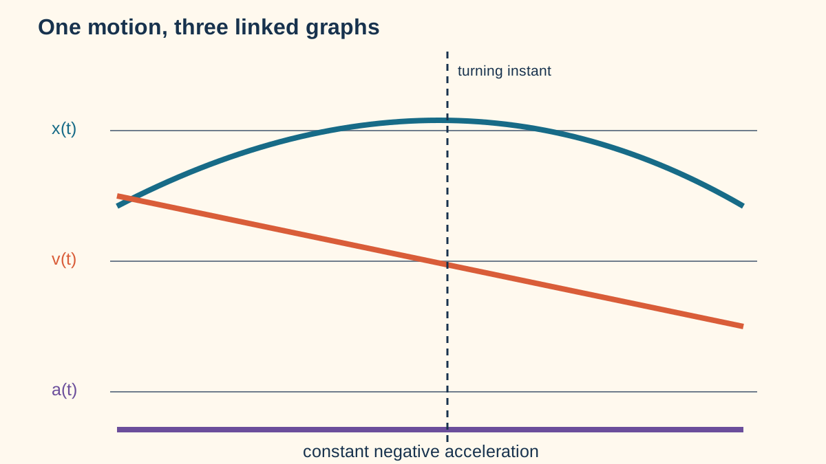
The graphs are not pictures of the path. Their vertical coordinates represent measured variables, and their shapes constrain one another.

Piecewise motion and sign

A horizontal segment on $x(t)$ means zero velocity. A horizontal segment on $v(t)$ means zero acceleration. A segment below the time axis on $v(t)$ means motion in the negative direction—not necessarily slowing down.

When velocity crosses zero, direction changes if the sign changes. Position has a local maximum or minimum at that instant, depending on how velocity changes sign.

Build a linear model

For approximately constant velocity,

In a linear fit $x=b+mt$, slope $m$ estimates velocity and intercept $b$ estimates position at $t=0$. Units are evidence: $m$ must have position/time units.

Worked example: constant-speed cart

Measured positions are $0.31$, $0.72$, $1.10$, and $1.51\text{ m}$ at $0$, $1$, $2$, and $3\text{ s}$. A fit gives

At $t=4.0\text{ s}$, the model predicts $1.90\text{ m}$. A prediction should be compared with a withheld measurement and its uncertainty.

Build a constant-acceleration model

For constant acceleration,

and

In a quadratic fit $x=c_0+c_1t+c_2t^2$, interpret $c_0=x_0$, $c_1=v_0$, and $c_2=a/2$. Coefficients require units: $c_2$ has $\text{m/s}^2$.

Worked example: cart released on an incline

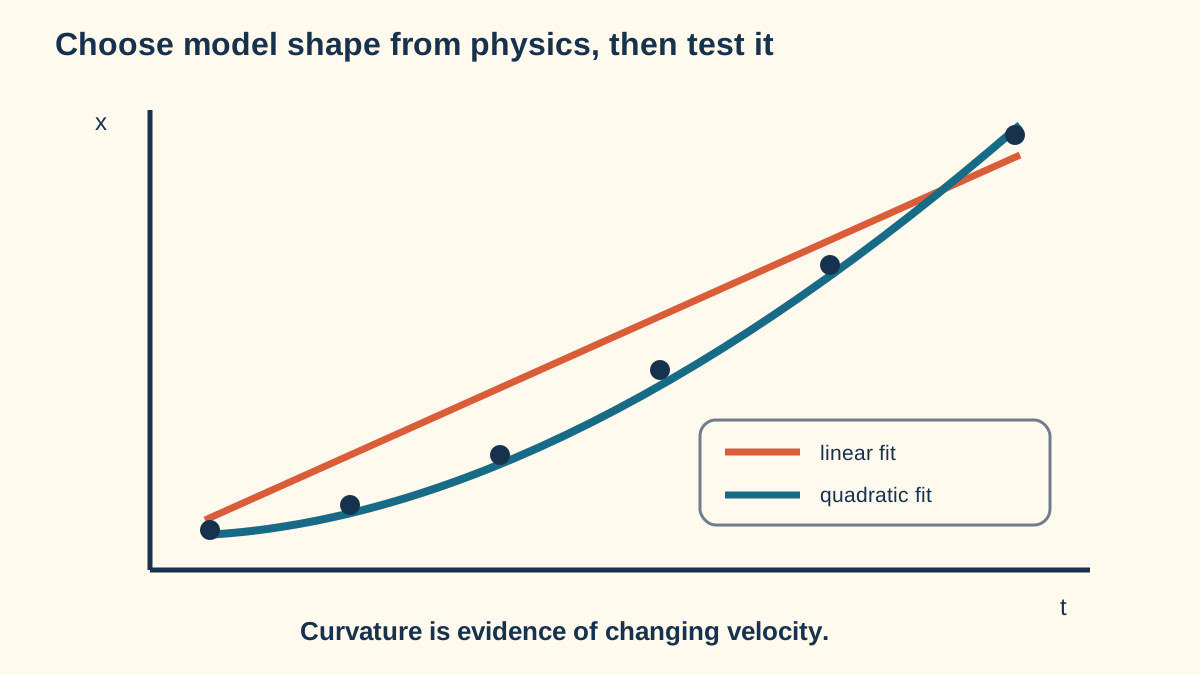
A quadratic fit gives

Therefore $x_0=0.020\text{ m}$, $v_0=0.080\text{ m/s}$, and

The factor of two is essential.

Residuals expose model mismatch

A residual is

For a suitable model, residuals should scatter around zero without a systematic pattern. Curved residuals from a linear fit suggest the motion is accelerating. A trend that grows with time may indicate a wrong model, timing bias, drag, changing acceleration, or calibration error.

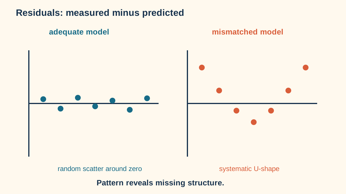
A large $R^2$ alone does not prove the physics model is valid. Inspect residuals, parameter units, uncertainty, model assumptions, and withheld predictions.

Slope from an interval

Average velocity over $t_1$ to $t_2$ is the secant slope:

Instantaneous velocity is approximated from a tangent or a sufficiently small symmetric interval. Making the interval smaller reduces curvature bias but can amplify measurement noise—a real experimental tradeoff.

Signed area from a velocity graph

Suppose velocity increases linearly from $-2.0$ to $+4.0\text{ m/s}$ over $3.0\text{ s}$. Its average value is $+1.0\text{ m/s}$, so displacement is

Distance is larger because the negative and positive regions must be added by magnitude after finding the zero crossing.

During learning: model audit

1. Identify each graph's variables and units.
2. Connect slopes and signed areas before selecting equations.
3. State the candidate model and physical assumptions.
4. Fit using only a training interval when testing prediction.
5. Inspect residual pattern and parameter uncertainty.
6. Evaluate withheld data and state the model's useful range.

Misconception clinic

“A motion graph shows the path.” It shows one variable versus another.

“A best-fit curve proves the model.” Fit quality must be tested with residuals, uncertainty, and prediction.

“Area below the velocity axis is negative distance.” It is negative displacement; distance uses magnitudes.

“The $t^2$ coefficient is acceleration.” It equals $a/2$ in the constant-acceleration position model.

“More decimal places mean greater accuracy.” Precision must reflect measurement and fit uncertainty.

After learning: retrieval and transfer

1. What do slope on $x(t)$ and area under $v(t)$ represent?
2. What residual pattern would challenge a constant-velocity model?
3. A quadratic coefficient is $-0.45\text{ m/s}^2$. What is acceleration?
4. Why should some data be withheld from fitting?
5. How can a small interval improve and worsen a slope estimate?

AP-style evidence routine

1. Define system, axes, origin, and interval.
2. Label measured variables and uncertainties.
3. Sketch expected graphs before fitting.
4. Fit a physically motivated model and interpret coefficients with units.
5. Inspect residuals and test a withheld prediction.
6. State the valid range, limitations, and alternative explanations.

Key takeaway

A mathematical model earns trust by connecting representations, producing physically meaningful parameters, leaving unpatterned residuals, and predicting data it did not fit.

Further learning and alignment

• College Board, “AP Physics 1: Algebra-Based Course,” https://apcentral.collegeboard.org/courses/ap-physics-1 (retrieved 2026-08-19). Alignment only; no endorsement.
• OpenStax, “2.3 Position vs. Time Graphs” and “2.4 Velocity vs. Time Graphs,” https://openstax.org/books/physics/pages/2-3-position-vs-time-graphs and https://openstax.org/books/physics/pages/2-4-velocity-vs-time-graphs (retrieved 2026-08-19). CC BY verification; no exercises copied.
• NIST/SEMATECH, “Residual Analysis,” https://www.itl.nist.gov/div898/handbook/pri/section2/pri24.htm (retrieved 2026-08-19). U.S. government statistical-model reference; no figures copied.