Lesson reading
live
55 min
Start with the lesson question, connect the representations, and test the model with evidence.
Inspect the opening phenomenon
Predict what changes, then name the evidence.
Apply in the lab
Name the evidence before reading the answer.
Read only what helps
Then use the lab and recall check.
More when needed
Transcript and resources stay available below.
Course progress
Odometry, Drift, and State Estimation
Decision challenge
Use the opening example to make a prediction, identify evidence, and explain which model supports it.
Predict motion, compare independent evidence, and correct according to uncertainty.
Predict motion, compare independent evidence, and correct according to uncertainty.
Lesson reading
live
55 min
Video script
draft
Transcript fallback
available
courses/ai-robotics/modules/07-localization-mapping-and-navigation/lessons/01-odometry-drift-and-state-estimation/video-transcript.md
Watch Drift Grow, Then Correct It
published
30 min
Mastery check
live
5 questions / 10 min
# Transcript A robot returns to its starting point, but odometry says it missed. Why? Odometry adds small motion estimates over time. It also adds wheel slip, scale error, and floor irregularities. Here, a tiny right-wheel bias bends the estimated path away from the true path. The estimator predicts from motion, compares that prediction with independent landmark evidence, then corrects the state according to uncertainty. The continuous odom frame is useful for control, even though it drifts. The map frame provides global correction and may jump. Predict, compare, correct—and always check time, frame, validity, and covariance. Which frame should a local controller follow? Practice the full drift-and-correction lab on EduQuest. ## V3 concise narration This robot returned to its starting point. But its odometry says it missed. How can both be true? Odometry adds thousands of tiny wheel rotations to estimate x, y, and heading. A little wheel slip looks harmless once. Integrated again and again, it bends the estimated path away from reality. A timestamped landmark gives independent evidence. The estimator predicts, compares, then corrects according to uncertainty. Quick check: which frame should stay smooth for local control—map or odom? Test your answer on EduQuest.
Reading lab
Connect the lesson's words, diagrams, graphs, evidence, and equations.
Odometry estimates motion relative to a starting pose. Every wheel rotation, visual feature match, or inertial update is slightly uncertain. Integrating those increments also integrates their errors, so the estimated path can gradually separate from the true path. State estimation manages that uncertainty by predicting motion, comparing the prediction with independent observations, and correcting the estimate.
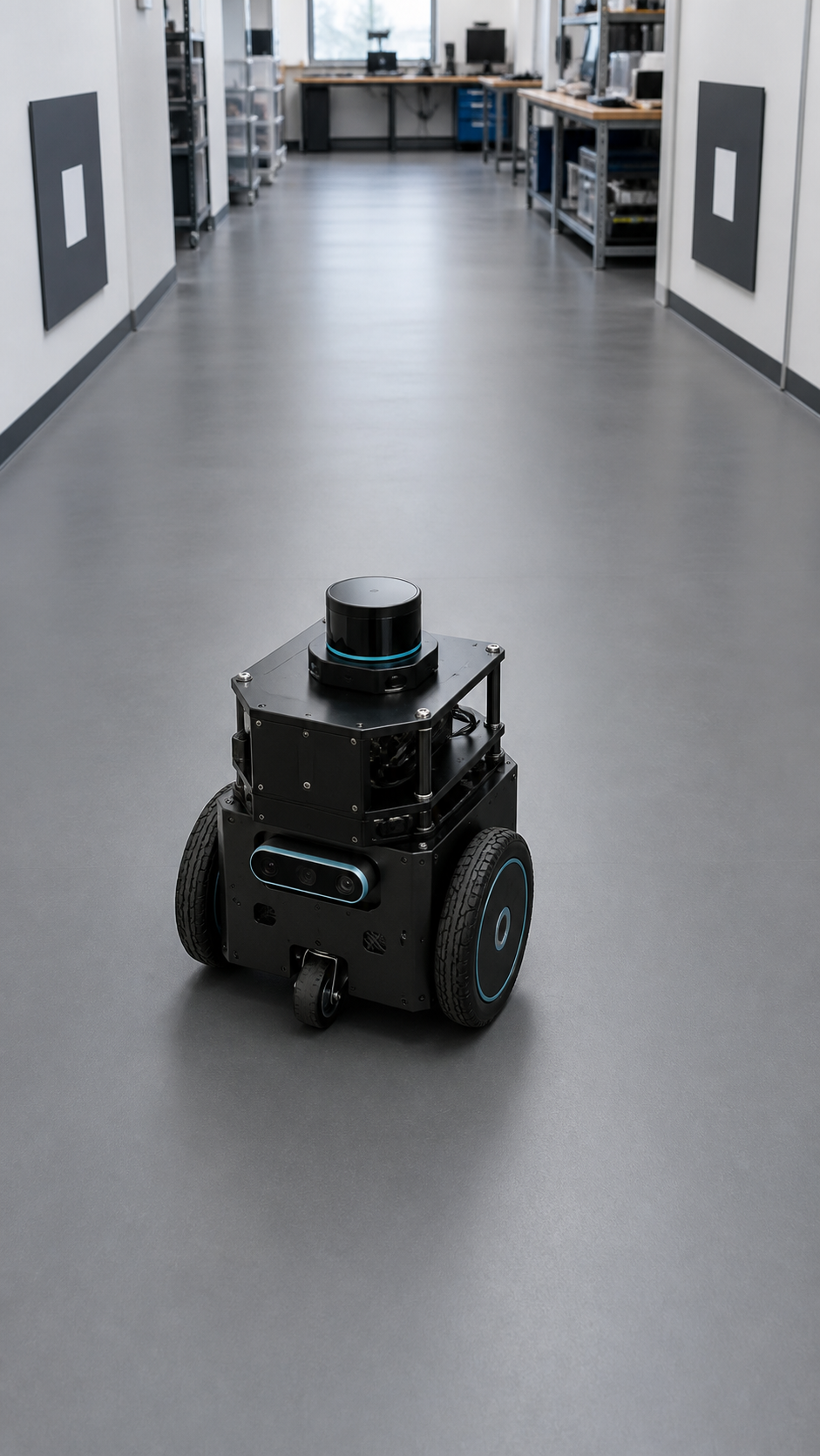
odom from globally corrected pose in map.Motion evidence draws a continuous pencil line. The robot predicts its next state from the previous state and the measured motion. A landmark observation is an eraser and ruler: it does not replace the whole drawing, but it can pull the estimate toward a pose supported by external evidence.
For a differential-drive robot with left and right wheel increments ΔsL and ΔsR, wheel separation b, and current heading θ:
Δs = (ΔsR + ΔsL) / 2
Δθ = (ΔsR - ΔsL) / b
x' = x + Δs cos(θ + Δθ/2)
y' = y + Δs sin(θ + Δθ/2)
θ' = θ + Δθ
The midpoint heading reduces curvature error for a small step, but it cannot remove incorrect wheel increments.
A robot has wheel separation b = 0.40 m. In one update the left wheel reports 0.20 m and the right wheel reports 0.24 m.
(0.24 + 0.20)/2 = 0.22 m(0.24 - 0.20)/0.40 = 0.10 rad, about 5.7°If the right wheel slipped and actually traveled only 0.21 m, the update invents both extra forward motion and extra rotation. Repeating small biased updates makes the path drift.
ROS REP 105 separates three useful frames:
| Frame | Meaning | Desired behavior |
|---|---|---|
base_link | Robot-fixed body frame | Moves with the robot |
odom | Locally consistent world frame | Continuous, accurate over short intervals, allowed to drift |
map | Globally referenced world frame | Long-term accurate, allowed to jump when localization corrects |
The typical chain is map → odom → base_link. Keeping local continuity separate from global correction prevents a sudden landmark update from looking like an impossible jump in wheel motion.
The nav_msgs/Odometry message carries pose and twist with covariance. Covariance expresses the estimator's uncertainty model. A small covariance does not prove correctness; an overconfident wrong sensor can damage fusion.
A robot drives straight, but one wheel radius is configured 2% too large. Predict the shape of the odometry error. Which observation could correct it, and what must match before fusion?
Odometry integrates relative motion and therefore accumulates error. A useful estimator preserves short-term continuity, represents uncertainty, and uses independent, correctly timed and framed observations to correct long-term drift. Diagnose localization by checking motion assumptions, timestamps, frames, covariance, and innovation—not only the final path.
Use a spreadsheet or short script to integrate wheel odometry, inject a realistic error, and apply landmark corrections. No robot hardware or paid software is required.
Create columns for step, left increment, right increment, estimated x, estimated y, estimated heading, landmark x/y, corrected x/y, and uncertainty score. Use wheel separation b = 0.40 m and start at (0,0,0).
0.20 m.1.02 to simulate radius miscalibration.0.04 m².corrected = 0.25 × predicted + 0.75 × observed for position. Label this as a teaching approximation, not a full Kalman filter.ΔsR - ΔsL.sin and cos.Learners who cannot use a chart can compare the numeric lateral error at steps 5, 10, 15, and 20 and describe its trend. The transcript and annotated visual convey the same mechanism without relying on motion or color.
odom remain continuous even when map is corrected?Run the same trace with unbiased wheels but a landmark observation delayed by two steps. Compare rejection, naive fusion, and acquisition-time transformation. Explain which result is defensible and why.